Statistical Learning Theory: VC Dimension, Structural Risk Minimization

Sometimes our models overfit, sometimes they overfit.

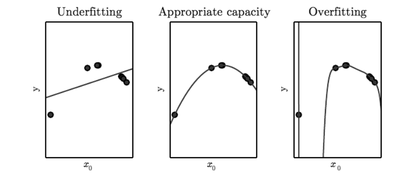
A model’s capacity is, informally, its ability to fit a wide variety of functions. As a simple example, a linear regression model with a single parameter has a much lower capacity than a linear regression model with multiple polynomial parameters. Different datasets demand models of different capacity, and each time we apply a model to a dataset we run the risk of overfitting or underfitting our data.

OK, so how do we know how well a model will perform our dataset without resorting to trial and error? What kind of theoretical guarantees do we have? Statistical learning theory is concerned with answering these questions.

(A note on terminology: selection in the hypothesis space, a selection in the function space, a family of functions, a model, etc. all mean the same thing for this post –  a function from inputs to classification outputs given some parameters.)

One of the best-known results from the field is as follows:

Suppose we’re evaluating a family of functions on our dataset with m training datapoints drawn i.i.d. from some distribution. With high probability (1 – ),

Test Error Train Error +

If you’ve spent time testing models under different datasets and this is new to you, it should be pretty remarkable. Without ever having tested your model on new datapoints to evaluate generalization, you have a (probabilistic) guarantee on the maximum error you will see when applying your model to new data!

But what’s H in this equation? H is the Vapnik-Chervonekis (VC) dimension, a measure of the capacity of a space of functions that can be learned by a statistical classification algorithm. In other words, the VC dimension quantifies the representational power of a function: a model with high VC can fit complex data in complex ways, while a model with low VC dimension will tend to underfit complex data. Informally, H increases as model complexity increases, and H is typically correlated with the number of parameters in your model (though there are notable exceptions on both ends of the spectrum).

How do we calculate the VC dimension for our model?

A function with parameter vector shatters a set of data points if, for all possible assignments of binary labels to those data points, there exists at least one parameter vector such that the function classifies the data points with no errors. The VC dimension is the largest number of points that can be arranged so that f shatters them. Note that we only require that a set of n points can be arranged in such a manner that they can be shattered – we don’t have to shatter any possible arrangement of the n points, just one. Although we only need one arrangement of points, remember that we will permute all possible binary labels across the points.

This is best explained with an example. Consider 2D space where we would like to separate datapoints with a hyperplane classifier: divide the plane with a line such that all labels are correctly classified. Does our classifier shatter 3 datapoints?

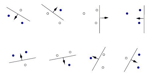
Yes! Well, what about 4? (Excuse the different image set, this is the neatest case of 4 datapoints I could find.)

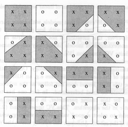
Nope! Look at the last two examples – it should be clear that we can’t separate these with a line such that all examples are correctly classified. You can try rearranging the points in the last two examples so that they can be linearly separated, but as a result one of the other labelings of those point will no longer be linearly classifiable.

Thus, the VC dimension of our family of line functions is 3 – plugging this back into the inequality above will tell us something about the maximum test error given our train error.

The game-like definition of shattering and just how it relates back to model evaluation seems a little obscure at first, but consider adjustments to model capacity:

Naturally, you can add more parameters to increase the VC dimension. In the case of the 4 datapoints above, adding more parameters like a few polynomials to our line classifier would enable us to shatter 4 points and will raise our VC dimension to at least 4. However, as our VC dimension goes up, so too does the rightmost term on our upper bound inequality:

Test Error Train Error +

…meaning the likely test error will increase. This checks back with our knowledge of underfitting and overfitting: adding parameters to our model tends to decrease training error (we can shatter more points) while increasing test error (due to overfitting on the train data).

How do we use the VC dimension to select a model that balances overfitting and underfitting?

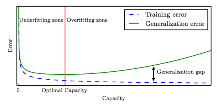
Structural Risk Minization gives us a principled way to search for and evaluate a family of functions. Quite simply, we can calculate the VC dimension and train error on multiple models and use the inequality above to determine the model of optimal capacity. What we obtain looks a lot like the well-known learning curve (above) rotated 90 degrees:

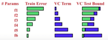
As we can see, number of parameters increase, train error decreases, VC dimension increases, and the result of our VC bound follows a parabola. In this case, f3 or f4 would be the optimal choice.

The VC dimension of a given model is quite difficult to ascertain, and differs depending on which variation of which model you’re using. You’ll have to look into the literature to determine the VC dimension for your model; for example, the VC dimension of neural networks.

Hopefully, you’re now armed with a new model selection method to employ alongside BIC, AIC, and cross-validation.